Making Decisions from Data with Percent RMS Statistics

Making Decisions from Data with Percent RMS Statistics

By Kelly Hile

Percent RMS - A useful tool for analyzing flow uniformity.

A typical day in the Airflow Sciences workplace is teeming with fluid dynamic data. One engineer is running a computer simulation of flow and heat transfer through industrial equipment. Another is conducting velocity and gas species testing of a scale model in our laboratory. Still another is standing next to a high pressure fan, collecting real-time flow measurements with precise instruments. In all of these cases, the output is the same: data.

Engineers are quick to collect data when designing a new system or troubleshooting an existing one. Whether the numbers come from a simulation or a physical instrument, designers routinely make key decisions based on large amounts of data. If we look at only the extremes (the high and low values) we might conclude that things are worse than they really are. If we look only at average values, we might miss problematic extremes or deviations. The method used for evaluating performance data matters as much as the accuracy of the data itself. That’s why in today’s blog we are highlighting one of our favorite data analysis methodologies – Percent RMS (or % RMS).

When it comes to airflow data in today’s industries, we are often looking at how uniform the flow profile is – this may refer to velocity, temperature, gas species, or other parameters of interest. Uniform flow means more consistent products, higher process efficiency, and improved equipment longevity. To illustrate this, we’ll walk through an example of a flow simulation using Computational Fluid Dynamics (CFD) where we want to achieve uniform velocity in a duct. Then we’ll take a look at how we use Percent RMS with data we measured in a client facility duct system.

Using Percent RMS with CFD Simulation Data

We ran a flow simulation of air flow through this duct system using Azore^®.

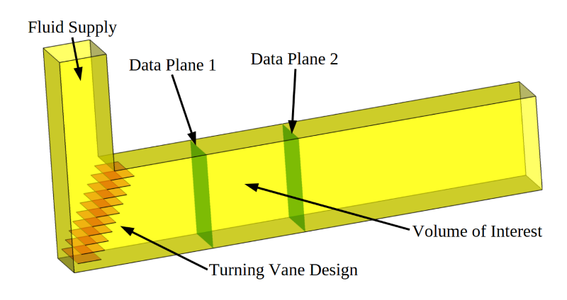
A 90-degree duct elbow that uses turning vanes to control the flow direction.

Air is supplied to the system as shown by the arrow labeled Fluid Supply. The goal of the simulation is to evaluate flow control devices in the 90-degree elbow to improve the fluid velocity uniformity through the Volume of Interest. For the purposes of this example, we’ll consider three simple design variations:

1. No vanes
2. A set of simple turning vanes (also called guide vanes) composed of horizontal flat plates
3. A reduced set of vanes (remove every other vane)

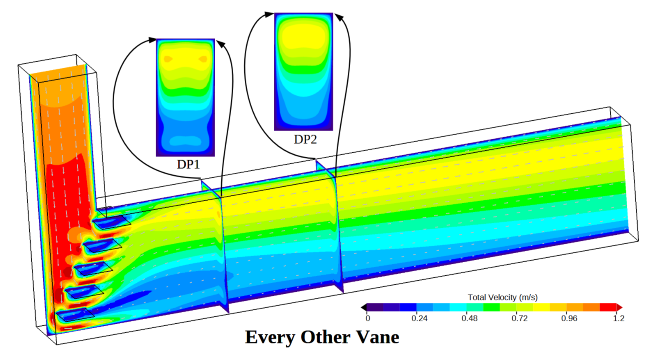
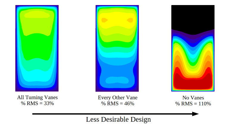
The images below show simulated flow predictions for each of these cases. Color contours of the total fluid velocity along the center line of the duct are shown for each design. Small vectors highlight the local direction of the fluid. The total velocity of the fluid passing through each data plane is pictured along with a normal projection view of these contour data.

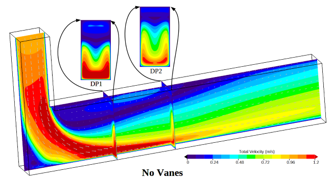
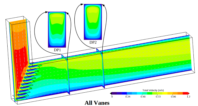
How should these three designs be evaluated? For this case, we are interested in the velocity passing through the Volume of Interest. With that goal in mind, we could choose to evaluate the fluid velocity uniformity as it passes through Data Plane 1 as the design criteria (labeled DP1 in the above images). One possible evaluation method is to simply display each normal velocity data plane side by side. A comparison like this is shown below for Data Plane 1. Visual inspection of these displays could be used to determine which design is better.

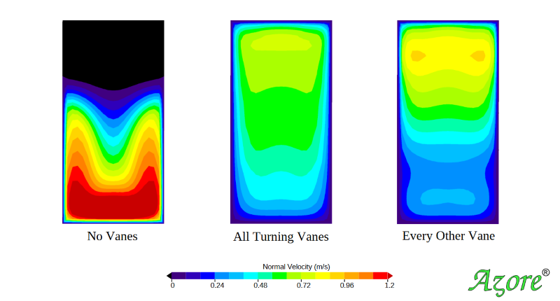
For some people looking at the simulation results, the best design will be obvious, while for others it may not be obvious at all. The people who can tell the difference between each design are performing a visual integration of the color contour fields. In other words, the result with more surface area color bands that are closest to the mean velocity will be the best design.

The visual inspection method has some problems. First, it lacks the ability to quantify each design. Furthermore, when two different designs result in similar contour fields, it can be difficult to determine which design is truly better than another. Another problem with visual inspection is that it can be impacted by the range used by the color bar. Consider if a very large color bar range is used. This choice will effectively reduce the number of color bands, making the results look more uniform. Conversely, if a tighter color bar range is used, it can make the variation seem significant.

For a thorough analysis of results, our engineers utilize statistics-based surface integration methods to calculate a single value. This value can then be used to quantify the velocity uniformity. There are many statistical values that quantify uniformity, and they go by many different names depending on the mathematics of the calculations and the industries where the values are used. We refer to this calculation as the Percent RMS, which is equal to the standard deviation (σ or s or SD) divided by the mean or average value (μ or ū or x̄) and expressed as a percentage. This statistical value goes by several other names, including Coefficient of Variation (COV or CV), Normalized Root-Mean-Square Deviation (NRMSD), relative standard deviation (RSD). A basic formula for Percent RMS is:

This is a good starting place to define %RMS, but depending on the measured parameter or the data under evaluation, weighting this calculation by area or mass might be prudent.

Simulation results can be easily used to determine statistical information since the colorful images are actually graphical representations of data distributed over a surface. This data can be used to calculate statistical data such as the Percent RMS of the velocity at the location of interest.

Let’s start by looking at the raw simulation data on Data Plane 1 for the Every Other Vane case. This data is shown on the left hand side of the image below. Here each sub grid face (f) is shown and colored by the normal fluid velocity (V_n) passing through that single sub grid face. The collection of these sub grid faces can be used to calculate the Percent RMS value for this surface using the equations shown to the right of the simulation data.

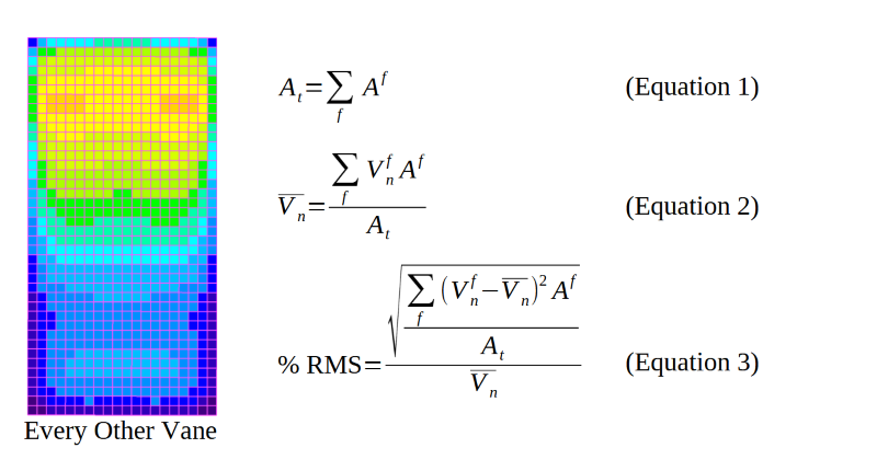
Equation 1 represents the total surface area of the data plane (A_t) by adding up the area of each sub grid face area. Equation 2 represents the area-weighted-average normal velocity (V_n) passing through the data plane. Equation 3 is the Percent RMS of the normal velocity for the data plane including the area weighting for each data point. The inclusion of the area weighting is critical for fluid dynamic analysis and is often an overlooked point. In “standard” statistical analysis, such as probabilities and mathematical surveys, a set of data may have equal weighting per data point. But in fluid dynamics and other engineering disciplines, the data points may not be equally distributed over a plane or surface of interest. This can occur when the CFD mesh does not have exactly equal sized cells at a plane (see the image below), or when experimental test data is not measured at spacially equal area locations in a flow stream. The area weighting (or in some cases mass-flow weighting) of the data becomes important in the analysis of flow uniformity via the Percent RMS calculation.

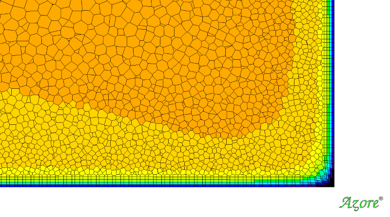
Area weighting the %RMS is especially important when the CFD mesh cells vary in size or when testing points are not evenly spaced.

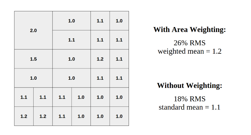
This example illustrates the importance of weighting by area when cells or test locations vary in size. Without area weighting, the large variation in the upper left corner is understated.

The Percent RMS calculation has specific benefits:

1. Its value becomes larger as the normal velocity distribution varies from the average normal velocity. Therefore, larger values will indicate less uniform velocity and smaller values will indicate a more uniform velocity. Zero Percent RMS represents perfectly uniform flow. This provides a single value that can be used to evaluate different designs.
2. As mentioned above, Percent RMS can account for variation in the mesh length scale, since the sub grid face area is used for the weighting. Using the weighted calculation means that the resulting value will be independent of the mesh length scale. Therefore, the same values will be reported for a coarse or a fine CFD grid.
3. Normalization by the average velocity passing through the data plane allows the Percent RMS value to be fluid flow rate insensitive. This allows the Percent RMS quantity to be used to evaluate uniformity even when the fluid flow rate might change in the system.

Most CFD tools provide some means for exporting the surface sub-grid face data. These data can then be imported into a spreadsheet and the Percent RMS value can be calculated using the provided equations. Our favorite CFD solver, Azore^®, conveniently provides these calculations directly in the user interface for rapid evaluation of flow uniformity in the model.

In the following image, the three designs have been sorted using the Percent RMS value calculated for each data plane. The left hand shows the most desirable design with a Percent RMS deviation of 33%, and the right hand side shows the least desirable design with a Percent RMS of 110%. Since each design has been assigned a single value, it is easy to see that adding vanes to the elbow has a pronounced impact on the velocity variability. The difference between the two vane designs, however, only indicates a secondary change in the velocity uniformity compared to the no-vanes case. This kind of information is key for real-world design decisions.

Besides allowing for apples-to-apples, direct comparison of different designs, the Percent RMS statistic also helps the engineer determine when a design meets performance objectives. For instance, if the goal of the above project required velocity uniformity of 50% RMS, then either vane design would be sufficient. The designer may choose the Every Other Vane concept as being less costly to install than the All Vanes concept. However, if the required velocity uniformity was 20% RMS, the CFD engineer would need to continue modeling of additional design concepts, to further improve flow uniformity. They may investigate more traditional, curved turning vane designs instead of the simple flat plates, replacing the square inside corner of the duct with a curved wall, or other more aerodynamic features.

Using Percent RMS with Testing Data

Aside from simulation results, our engineers also use Percent RMS to evaluate real-world data from flow measurements we perform at client sites. Consider the velocities our team measured in two ducts (east and west) at an industrial plant to assess fan performance. We used our state-of-the-art flow measurement system, the 3DDAS, to measure the 3D velocity profile at multiple points across one location in each duct. The resulting velocity data can be visualized by color, where each individual box represents a velocity probe sampling location.

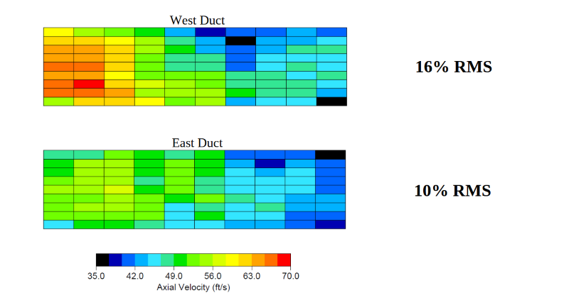
The % RMS calculation gives a single point of comparision between these two ducts, the West Duct experiencing a higher variation in flow velocity.

Additional Applications

Applicable to more than velocity uniformity, but use with caution.

The Percent RMS methodology is not limited to velocity data, and can also be applied to other measurement parameters. For example, for industrial processes where chemical injection and mixing is important, the mixture uniformity can be examined via Percent RMS statistics. This is common in pollution control equipment design such as Selective Catalytic Reduction (SCR) systems. An SCR is an industrial version of an automobile catalytic converter, and is used to remove nitrous oxides (NOx) emissions from combustion gases at power plants, refineries, and other industrial facilities, minimizing release of NOx to the atmosphere. Ammonia (NH3) is injected into the gas stream in small quantities, mixed with the NOx, and converted to harmless Nitrogen (N2) and water vapor (H2O) through a catalyst. The NOx removal is optimized when the Ammonia-to-NOx uniformity is very good, 5-10% RMS if possible.

Whereas it was previously noted that velocity uniformity should be calculated as an area-weighted statistical value, a gas species like ammonia or NOx should consider the Percent RMS calculated in a mass-weighted manner. This is because gas species are generally denoted in CFD simulations or field measurements as a concentration (mole fraction, ppm, ppb, etc.), while often the important uniformity parameter for a chemical process is related to the mass flow or stoichometric mixture ratio at a plane of interest or through a volume of interest.

The CFD model below evaluates an SCR installed downstream of a Heat Recovery Steam Generator (HSRG). Ammonia is introduced at the Ammonia Injection Grid (AIG) just upstream of a catalyst layer. Engineers at Airflow Sciences improved the design of the SCR by modifying the injection grid and moving it more upstream. Prior to the redesign, the CFD model showed a 69% RMS variation in NOx concentration, weighted by mass. The design modifications improved the concentration uniformity to 7% RMS. More uniform performance over the bed of the catalyst can prolong catalyst life and reduce ammonia slip, a common issue with SCRs.

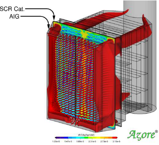
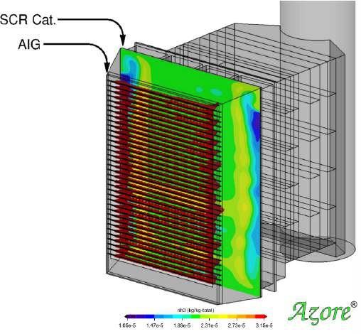
A CFD model of an SCR shows 69% RMS in NOx concentration (left). After a redesign, this is reduced to 7% RMS (right). The Percent RMS is weighted by mass rather than area when evaluating species concentration.

When dealing with a collection of measurements, the Percent RMS calculation can help assess overall process performance and quantify improvements. When designing or modifying a process with CFD data or test data, having a common way to evaluate and compare datasets will drive good decision-making at all process levels.

At Airflow Sciences, we’ve been solving flow-related problems since 1975 in all kinds of industries. Contact us today too see how we can improve your business with CFD modeling, lab, or test support.